The Blind Source Separation (BSS) [1] technique aims to recover N statistically independent source signals from M mixed signals. Here, "blind" means that the prior knowledge of the source signal and the mixed channel is unknown. Due to this "blind" nature, BSS is widely used in digital communications, array signal processing, speech and image processing. The linear instantaneous hybrid model is one of the most common models in the BSS problem. It is suitable for environments such as remote communication. This model is also the basic model of other hybrid models (such as convolutional blending). The mathematical description is as follows:
 Where A is the unknown mixing matrix, t is the sampling instant, s(t)=[s1(t),...,sN(t)]T is a vector of N unknown statistically independent source signals, x(t)= [x1(t),...,xM(t)]T consists of M available mixed signals, n(t)=[n1(t),...,nM(t)]T contains M-channel additive white Gaussian noise. At this point, the BSS problem translates to finding a de-mixing matrix W such that the output y(t) = Wx(t) is an estimate of the input s(t) and allows for uncertainty in the magnitude and ordering.
In order to solve the above problems, many effective methods have been proposed, such as independent component analysis [2], nonlinear principal component analysis [3], etc., but most of these methods require the number of known source signals, and generally It is assumed that the number of source signals is equal to the number of mixed signals, that is, M=N. In practical applications, such settings are often unsuccessful, because the number of source signals is often not directly available as source information, and may even be dynamically changed. For example, in a wireless communication system, the number of users accessing the system may be at any time. Are changing. It can be seen that in practical applications, M=N is difficult to satisfy. When the number of sensors that receive the mixed signal is set to be sufficient, the over-determination of M>N often occurs. For the BSS problem where the number of sources is unknown and under the overdetermined assumption, the literature [4] first estimates the number of sources in the whitening stage.  And then reduce the mixed signal dimension M to
  The natural gradient algorithm is used to solve the above BSS problem, but when the mixing matrix is ​​ill-conditioned or the amplitude ratio of the source signal is out of balance, the algorithm may fail. The literature [5] theoretically proves that the minimum mutual information criterion can be used in the case of overdetermination, and proposes an improved natural gradient algorithm suitable for the number of unknown sources. In [6], the neural network of self-organizing structure is used to estimate the number of instantaneous source signals, and the size of the neural network is adjusted to separate the mixed signals. Literature [7] proposed an adaptive neural algorithm (ANA) to further improve the stability of convergence, but the convergence speed is slower. In [8], a momentum term is added to the ANA algorithm, and a Neual Network with Momentum for Dynamic Source Number (NNM-DSN) algorithm is proposed. The algorithm converges more quickly. Fast and steady-state error is smaller. However, the above algorithms generally do not consider noise, and the degree of practicality of the algorithm is not high.
In this paper, a new online blind source separation algorithm is proposed for the BSS problem under noisy dynamic source conditions. The algorithm consists of two parts: the first part is based on the minimum description length (MDL) [9]. Dynamic source number estimation algorithm, which can accurately estimate the number of instantaneous sources in the channel in real time; the second part is a variable-step neural network algorithm based on deviation removal. The algorithm uses a feedforward neural network structure and is added to the learning criterion. The deviation removal term caused by noise is given, and a variable step size strategy is given on this basis. Simulation experiments show that the proposed algorithm can accurately recover the source signal under the condition of noisy static source and dynamic source. Compared with ANA algorithm and NNM-DSN algorithm under noise, the algorithm is based on static source and dynamic source. The performance is better, the convergence speed is faster, and the steady-state separation performance is close to the performance of the NNM-DSN algorithm in the case of no noise.
1 Introduction to the algorithm
For BSS problems with noisy dynamic sources, the number of instantaneous source signals must first be determined.  And then reduce the dimensions of the mixed signal vector to
  Dimension, where M-
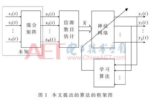
  The highly correlated components will be removed to adjust the size of the neural network, so that the problem becomes a noisy BSS problem with the number of source signals and the number of mixed signals. Using the variable-step-based neural network algorithm based on bias removal proposed in this paper. An estimate of the source signal is obtained. Figure 1 shows the framework of the algorithm, in which the neural network and the learning algorithm work together to achieve the separation of the mixed signals. The source number estimation and mixed signal separation methods will be separately described below.
1.1 Estimation of source number
For the estimation of the instantaneous source number of dynamic sources, the literature [7] uses an improved cross-validation algorithm; the literature [8] eigen-decomposes the mixed-signal covariance, and uses the structure of the eigenvalues ​​to estimate the number of source signals. However, the above algorithms are used in noiseless conditions. Some classical batch source estimation algorithms (such as MDL) can be used in noisy situations. Therefore, based on MDL, a dynamic source number estimation algorithm is proposed to accurately estimate the number of sources in the channel in real time.
The mixed signal value at the current time and the previous B-1 time is used to estimate the number of source signals at the current time, and the instantaneous covariance matrix at time t is defined as:
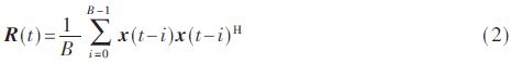
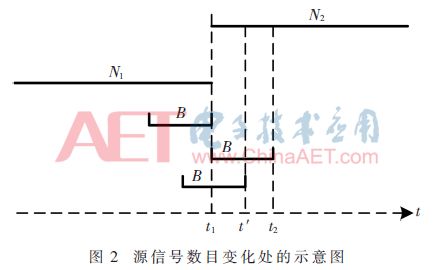
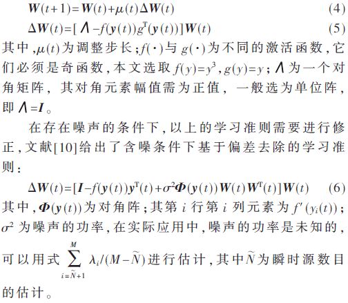
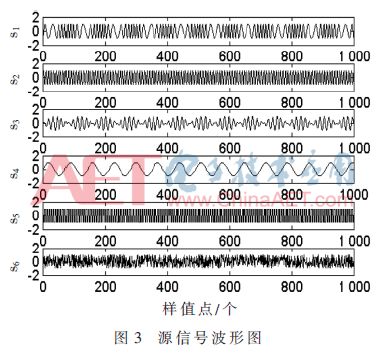
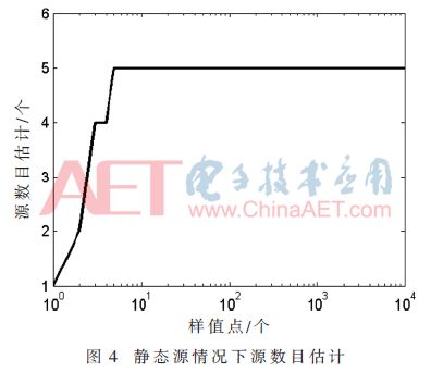
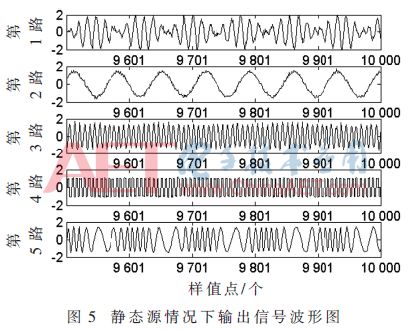
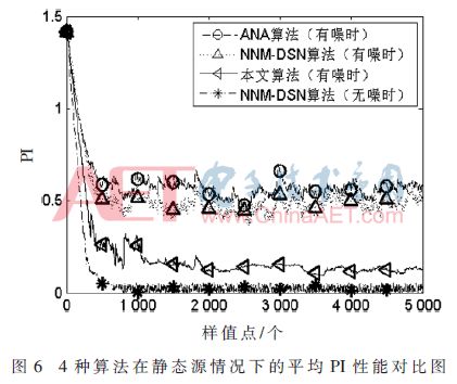
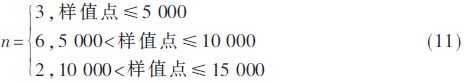
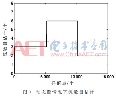
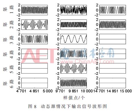
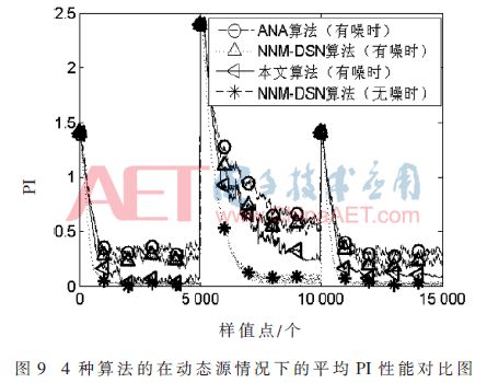
Among them, the superscript H represents the conjugate transposition operation, t ≥ B. When t Where σ2 is the power of the noise, the number of instantaneous source signals at the current moment can be estimated by using the MDL detection criterion. There is a problem in estimating the number of instantaneous source signals by the above method, that is, a small overestimation occurs when the number of source signals changes. Figure 2 shows a schematic diagram of the change in the number of source signals. N1 is the number of signals before the number of source signals changes, N2 is the number of changed signals, and t1 is the critical point at which the number of source signals changes. At the first B-1 moments of the time, the number of source signals remains stable, so the number of source signals can be accurately estimated to be N1 by the above method. The time t2 satisfies t2-B+1=t1, and the number of source signals remains stable at the first B-1 time, so the same reason can accurately estimate the number of source signals as N2. At the time between t1 and t2, such as t', the number of source signals may be overestimated, but since the time difference between t1 and t2 is less than B, the duration of such overestimation does not exceed B. In order to solve the above problem, the algorithm starts recording the current estimated source number value when detecting the change of the number of sources, and after the γB (1<γ≤1.5) time thereafter, if the estimated source signal changes, the first change is The source number value between the second changes is changed to the source number value before the first change, and then the recording is started from the time when the second source number changes, and the above detection is repeated until the γB time period after the recording start time If the value of the estimated source number does not change, the recording is stopped and the next estimated number of sources is changed. In this way, the overestimation problem at the source number conversion can be eliminated. 1.2 Separation of mixed signals In general, the element wij of the de-mixing matrix is ​​considered to be the weight of the neural network, which can be adjusted by the gradient descent method. This paper considers a robust learning criterion based on feedforward neural networks. The expression is as follows: Substituting equation (6) into equation (4) can obtain a neural network algorithm based on deviation removal, but the step size μ(t) in the algorithm must be properly selected. If μ(t) is too small, the convergence speed is too slow; Then the steady state fluctuation is too large. In order to overcome the above problems, a variable step size strategy is introduced. Referring to [11], μ(t) can be adjusted by the following recursion: 2 Simulation experiment In order to verify the performance of the proposed algorithm under noisy dynamic source conditions, this paper will compare with the ANA algorithm in [7] and the NNM-DSN algorithm in [8]. The selection of the source signal is consistent with that in the literature [7-8]. The sampling rate is set to 1 kHz. The waveform diagram of the source signal is shown in Figure 3. The mixing matrix A is randomly generated, as long as the full rank is satisfied. In this paper, the performance index [2] is used to evaluate the separation performance of the algorithm. The smaller the PI, the better the separation performance. The simulation experiment includes two cases, one is the case of a static source, and the other is the case of a dynamic source. All experiments will be performed 100 times Monte Carlo test. In the following experiment, n=k(k≤6) means that the first k signals in Fig. 3 are taken as the source signals, and B=200, γ=1.2. 2.1 Static source situation In this section, consider the case of static sources. Let n=5 remain unchanged, the number of receiving sensors is 8, take 10 000 sample points, and the Signal-to-Noise Ratio (SNR) is set to 10 dB. Figure 4 shows an estimate of the number of sources using the algorithm in the case of a static source. It can be seen that the algorithm quickly obtains an accurate number of sources. Figure 5 is a waveform diagram of the output signal obtained by the algorithm in the case of a static source. The figure shows the last 500 output sample points. As can be seen from the figure, the output signal completes the recovery of the source signal, and only the amplitude and the order are present. Uncertainty. Figure 6 is a comparison of the average PI performance of the ANA algorithm, the NNM-DSN algorithm, the proposed algorithm, and the noise-free NNM-DSN algorithm under static conditions in the presence of noise, where the NNM-DSN algorithm is used for performance without noise. According to the figure, when the noise exists, the performance of ANA algorithm and NNM-DSN algorithm deteriorates and the stability decreases. The average PI performance of the proposed algorithm is better than the ANA algorithm and NNM-DSN algorithm under noisy conditions, and is close to no noise. The performance of the NNM-DSN algorithm is faster than that of the ANA algorithm and the NNM-DSN algorithm in the noisy case. 2.2 Dynamic source situation In this section, consider the case of dynamic sources. Let n=3,6,2 and take 15 000 sample points. The specific settings are as follows: Let the signal-to-noise ratio be 10 dB and the number of receiving sensors be 8. Figure 7 shows the source number estimation of the algorithm in the case of dynamic source. It can be seen that the number of sources is quickly and accurately estimated. Figure 8 is the waveform diagram of the output signal obtained by the algorithm in the case of dynamic source. The last 300 sample points of the separated signal in the case of three different source numbers, wherein the blank box indicates no output, it can be seen that the mixed signal is successful. Ground separation, there is only uncertainty in the magnitude and order. Figure 9 is a comparison of the average PI performance of the ANA algorithm, the NNM-DSN algorithm, the proposed algorithm, and the noise-free NNM-DSN algorithm in the presence of noise in the presence of noise. Similarly, the NNM-DSN algorithm is used when there is no noise. For performance reference, when the number of sources changes dynamically, all algorithms can adjust to convergence. ANA algorithm and NNM-DSN algorithm have average PI qualitative deterioration in noisy conditions, and ANA algorithm and NNM-DSN algorithm in noisy conditions. In comparison, the average PI performance of the proposed algorithm is better and the convergence speed is faster, and the average PI performance at steady state is close to that of the NNM-DSN algorithm when there is no noise. 3 Conclusion In this paper, a new online blind source separation algorithm is proposed for the noisy dynamic source. It consists of two parts: the dynamic source number estimation algorithm based on MDL and the variable step size neural network algorithm based on deviation removal. The new algorithm can accurately estimate the number of instantaneous source signals in real time and successfully separate the mixed signals under noisy conditions. The simulation experiments show that the proposed algorithm can accurately recover the source signal under both the noisy static source and the dynamic source. Compared with the ANA algorithm and the NNM-DSN algorithm in the noisy case, the proposed algorithm has better separation performance and Faster convergence speed and separation performance close to the performance of the NNM-DSN algorithm in the absence of noise.
Android is an open source mobile operating system based on Linux platform released by Google at the end of 2007, and then improved for use in netbooks and MIDs. The platform consists of operating system, user interface and application software, and is claimed to be the first truly open and complete mobile software for mobile terminals.
To put it simply, the Android system is actually a very open system. It can not only realize the functions of the most commonly used notebook computers, but also realize various directional operations like mobile phones. Moreover, it is specially designed for mobile phones. The operating system developed for equipment has advantages in system resource consumption and human-computer interaction design. It is an operating system that combines traditional and advanced advantages.

New Android Tablet,Android Tablet,New Android Tablet
Jingjiang Gisen Technology Co.,Ltd , https://www.jsgisengroup.com